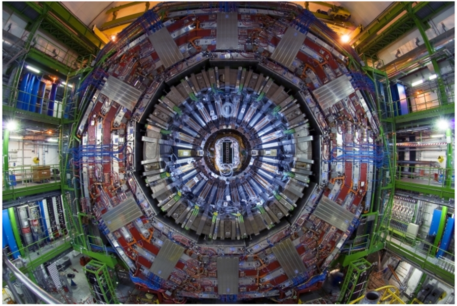
Quarks and gluons are the elementary particles that make up protons and neutrons, which are in turn the building blocks of the nucleus of every atom. Gluons are the particles that mediate the strong nuclear force, which is responsible for “gluing” the quarks together in protons and neutrons. The interaction between quarks and gluons is described by quantum chromodynamics (QCD), the quantum theory of the strong nuclear force. While quarks and gluons are not directly observable, we have ways of studying them without direct detection. We can use jets, the collimated streams of particles produced in high-energy collisions, as a proxy for the energetic quarks or gluons created in a collision. Thanks to this association, we have studied the strong force at distances as short as 10-20 meters (that’s 19 zeroes after the decimal point!). Jets have been used to extract fundamental parameters of the standard model, search for physics beyond the standard model, or to characterize the hot and dense medium created in ultrarelativistic heavy ion collisions.
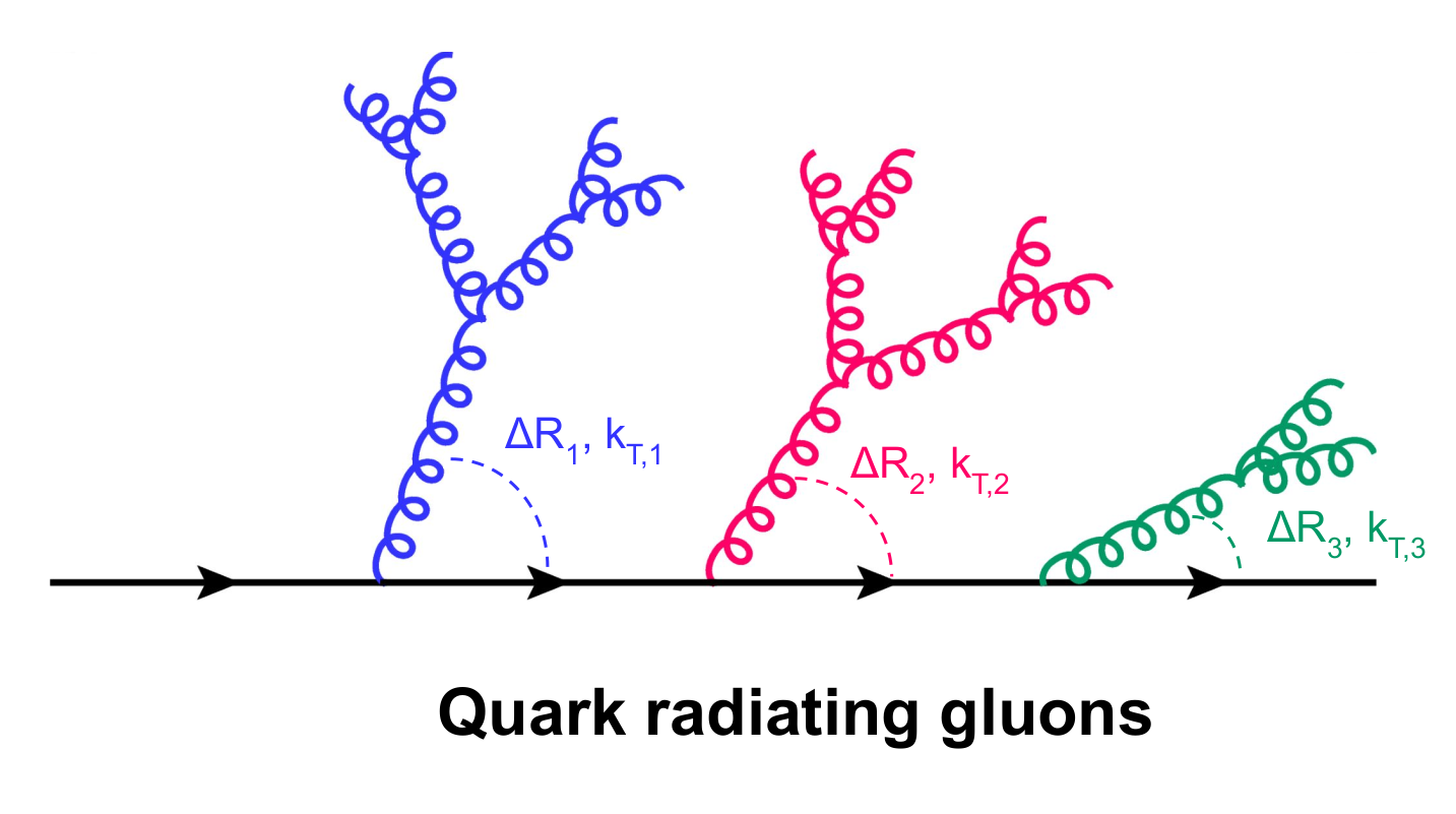
In recent years, we have learned that valuable information about the strong force lies in the structure of jets themselves. To get an insight into how the basic rules of QCD radiation are connected to the structure of a jet, let us consider the radiation of gluons from a quark, as shown schematically in Figure 1. To quantify the hardness of a kick received by a radiated gluon, one can use its transverse momentum relative to the recoil quark, which we denote by kT, and the opening angle of the branching, denoted by ΔR. The probability for a quark to emit a gluon with a given kT and ΔR is approximately given by ⍺s / (kT ΔR), where ⍺s is the strong coupling constant, which quantifies the strength of the strong interaction. According to this expression, gluon emissions are preferentially “soft” (low kT) and “collinear” (small ΔR). This particular dependence of the emission probability is a consequence of a fundamental property of Nature, known as “scale invariance”: at high energies, the strong force is (approximately) the same at every distance scale.
To visualize the kinematics of these emissions in a two-dimensional plane, it is intuitive to use kT and ΔR for the vertical and horizontal axes. We can go one step further and use functions of kT and ΔR to make the properties of scale invariance pop up more clearly. For instance, emissions are distributed uniformly when using the logarithm of kT and the logarithm 1/ΔR for the vertical and horizontal axes, as in Figure 1. This space, known as the Lund plane, is a powerful visualization tool of QCD radiation.
 |
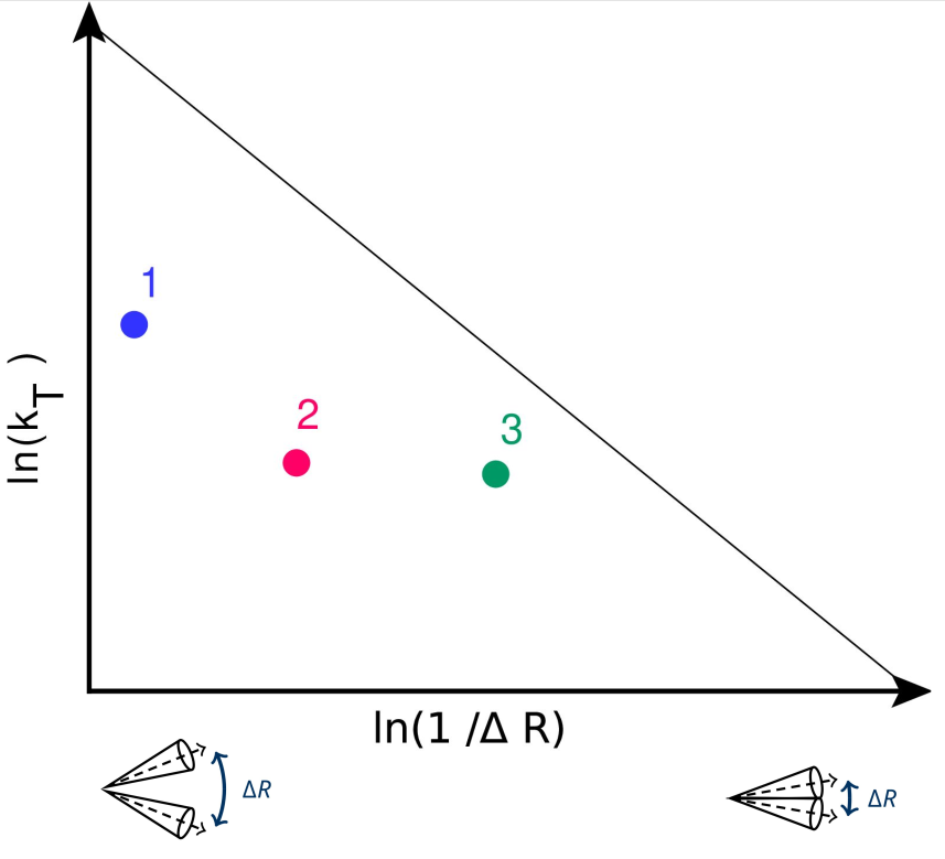 |
Figure 1: Left: Gluon emissions (rungs) from a quark. Right: The splitting angle ΔR and transverse momentum kT of the emissions fill a two-dimensional logarithmic plane known as the Lund plane. The emissions are filled from large to small ΔR, from left to right, following the angular ordering expected from color coherence.
Since the emission probability is nearly the same at every kT and ΔR, one can imagine using this as a rule to iterate 1→2 branchings to build a fractal tree of quarks and gluons: a jet. This fractal-like pattern of emissions is an approximation, which is broken mainly by two mechanisms. One is that ⍺s “runs” with energy, a quantum mechanical effect induced by the presence of virtual quarks and gluons popping in and out in the vacuum. The other has to do with the confinement of quarks and gluons in hadrons. Still, the foundational pillar of the structure of a jet is a consequence of the approximate scale invariance of the strong force.
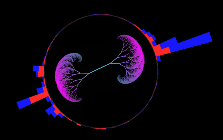
While we have a theoretical grasp of how a jet is formed, it is not straightforward to expose this fractal-like pattern of emissions in practice. Experimentally, we do not directly see quarks and gluons; jets are collections of tracks and calorimeter signals in our detectors. The challenge is analogous to trying to infer the branches of a tree by only looking at its leaves, as illustrated in Figure 2.
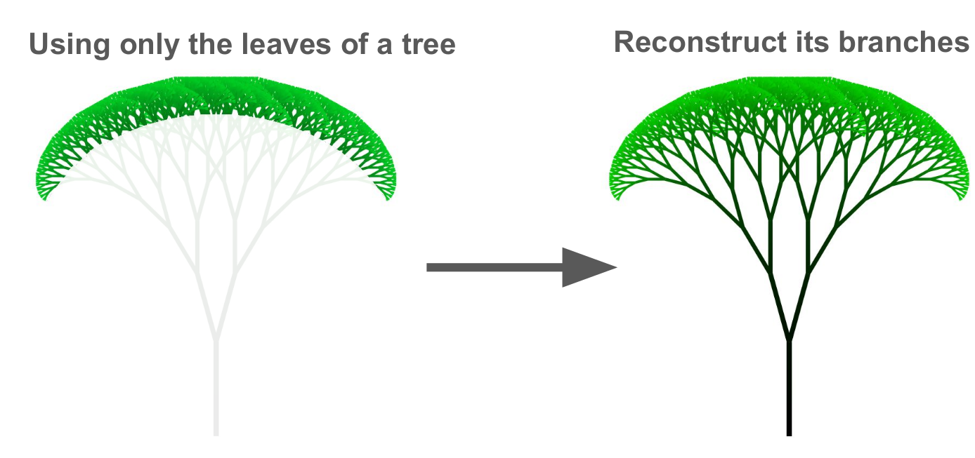
Figure 2: What experimentalists want to do is analogous to reconstructing the branches of a tree based only on its leaves.
In this spirit, theorists proposed to use a sequential clustering algorithm (known as the Cambridge/Aachen algorithm) to construct a hierarchical tree of emissions to analyze the radiation pattern of the jet in the Lund plane: the Lund jet plane. We can follow the jet clustering history in reverse and analyze the jets within the jets, which can be used as proxies for the quark and gluon emissions in the jet in a theoretically well-motivated way.
 |
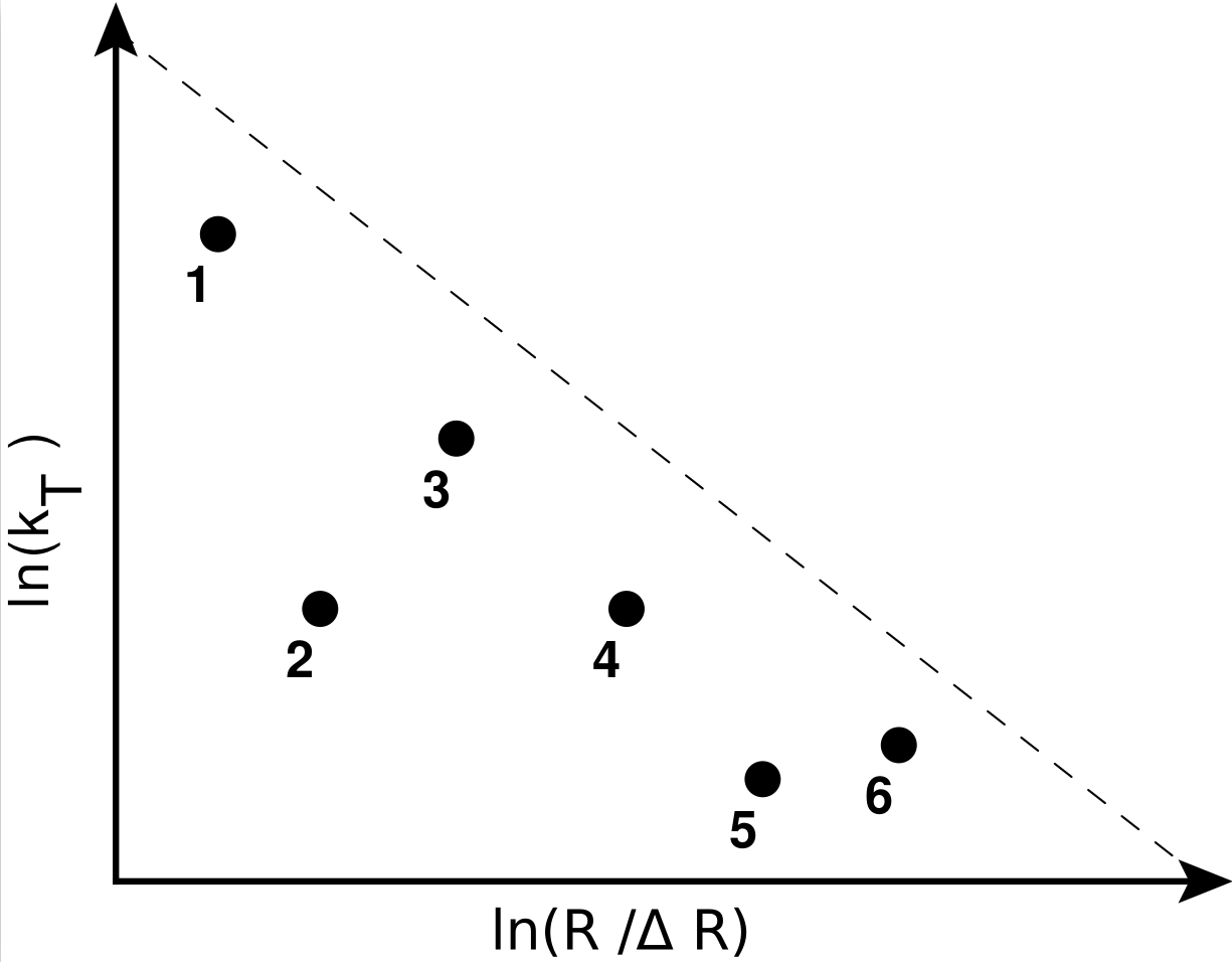 |
Figure 3: Left: Schematic diagram of the jet declustering tree; the numbers represent the order of appearance of the emissions in the declustering. Right: The corresponding Lund jet plane.
Following this prescription, CMS measured the primary Lund jet plane density of emissions using proton-proton collision data collected during Run-2 (2016–2018) at a collision energy of 13 TeV. The measurement is done for jets with transverse momenta greater than 700 GeV. This high transverse momentum selection is not a usual choice for CMS analyses but it is necessary to have hard emissions inside the jets. Since jets are roughly cone shaped, we can identify an effective cone radius R measured in units of rapidity and azimuthal angle. Jets with R = 0.4 and R = 0.8 were used; they are sensitive to different aspects of the jet formation. The measured observable is the average density of emissions in the Lund jet plane. At a first approximation, this observable is proportional to ⍺s. Jets with transverse momenta at the TeV-scale can have emissions inside of them with kT as large as 700 GeV.
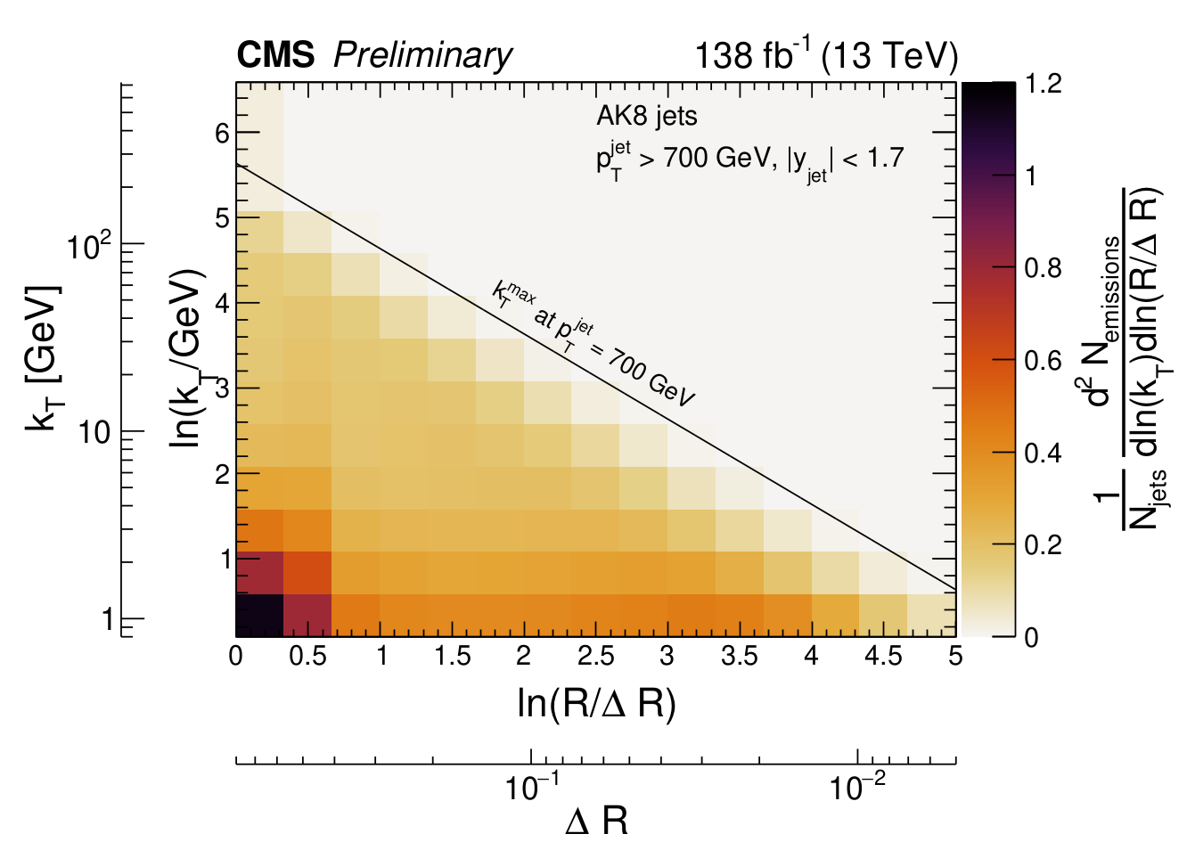
Figure 4: Primary Lund jet plane density of jets with a radius R = 0.8. The density of emissions increases at low kT, whereas it saturates at high values of kT, following the running of the strong coupling constant ⍺s.
For the data to be useful to theorists and other experimentalists, the distributions are corrected to remove all the detector effects using a statistical procedure known as “unfolding”. According to Cristian Baldenegro, one of the leading contributors to this analysis, the unfolding correction is the most crucial and delicate aspect of the analysis. The two-dimensional unfolded distribution for R = 0.8 jets is shown in Figure 4. The Lund jet plane helps us visualize the phase space of radiation inside the jet. The measurement allows us to see which aspects of the theoretical calculations of the parton branching and hadronization need to be improved.
This precision measurement places us one step forward in understanding the formation of jets at a fundamental level, a key ingredient in our understanding of Nature at subatomic distances.
Read more about these results:
- CMS Physics Analysis Summary: Measurement of the primary Lund jet plane density in proton-proton collisions at 13 TeV
-
@CMSExperiment on social media: facebook - twitter - instagram
- Do you like these briefings and want to get an email notification when there is a new one? Subscribe here