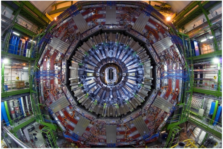
, a muon (in red), and an energy imbalance in the transverse plane (the purple arrow).")
Even if the standard model of particle physics (SM) describes Nature incredibly well, it fails in providing insight to a number of observations such as the existence of dark matter. How do we get a better (and bigger) model than the SM? From the experimental point of view, two approaches are common ground: the first path implies a big adventure, that of searching for new particles that don’t fit in the SM, such as the aforementioned dark matter; a different way to break the SM is what we call precision physics, meaning that we aim at measuring known things with ever increasing precision. The better the experimental precision is (i.e., the smaller is the measurement uncertainty), the more we can challenge the SM.
Following the precision physics path, one can measure how often different processes (different sets of particles) are produced in the proton-proton collisions taking place at the LHC. Our scientific and quantitative definition for this “how often a process is produced” is the cross section. And out of the many processes that are produced at the LHC, we focus our analysis on the production of two W bosons, one of the particles carrying the electroweak (EW) interaction. This process is of enormous interest for many reasons, among them the fact that it is sensitive to the properties of EW bosons self-interactions, and provides a powerful test of predictions related to both the quantum chromodynamics (QCD, the theory of strong interactions) and the EW components of the SM. These W bosons cannot be observed directly in our detector, as their lifetime (the time it takes since they are produced until they decay to lighter particles) is too short. So, we detect their decay products; like detectives, we use the decay products to infer their “mother particles”. The W bosons can decay in several different ways, but the choice is clear if we look for a clean measurement with little background noise: we want to reconstruct one W boson decaying to an electron and its corresponding neutrino, and the other decaying to a muon and its corresponding neutrino. Neutrinos cannot be detected in CMS, but their presence can be inferred by applying conservation laws: we evaluate their energy as the energy that is “missing” with respect to the value that we know must be there, given the energy of the initial collision. We basically select proton-proton collisions that produce an energetic electron-muon pair, together with a large amount of missing energy.
The WW production cross section is known with excellent precision from previous measurements at lower energies. Can the higher energy of the LHC collisions lead to something new? The selection of events with an energetic electron-muon pair plus missing energy is not enough, as the amount of background processes is still way above our signal count. We need to apply a more stringent selection that heavily depletes the background level (call it noise reduction) and keeps as much signal as possible. In any case, even the best and most perfect selection will remove some signal events and keep some background noise. How do we know, in this situation, what the WW cross section is?
We perform this analysis by looking at proton-proton collisions with a total energy of 13.6 TeV and we include all the data collected by the CMS detector in 2022. Figure 1 shows all the events that pass the signal selection, as a function of how many jets they have. One can immediately see that the majority of events have zero jets. The measured data (the real collisions) are represented by the black circles. The SM predicts that the different coloured histograms (different processes) should account for the measured data points. This is true, as can be seen in the lower part of Fig. 1, which shows that the data over SM ratio is compatible with unity for all the bins. Out of the processes represented, we are interested in the light blue one, the WW production. The magnitude of this process is left free in a fit that tries to find the best agreement between the data points and the sum of all histograms. The result of the fit is also shown in Figure 1.
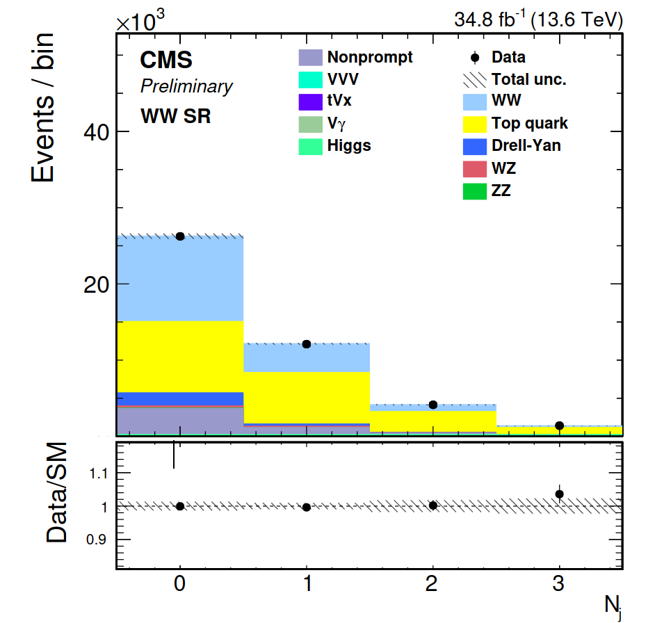
Figure 1: Yield of WW candidate events as a function of the number of reconstructed jets (top panel) and the corresponding ratio to the SM prediction. The gray bands (vertical bars) represent the uncertainties in the predicted yields (in the data).
The measured inclusive cross section is 125.7 ± 5.6 pb, which is consistent with the theoretical prediction of 128 ± 3 pb. So, there is agreement at the level of the integrated (inclusive) value, but what about a more detailed comparison? Can the SM also correctly predict the variations with jet multiplicity? The result is shown in Fig. 2, which compares the SM prediction with the measurement (after subtracting the estimated backgrounds and accounting for detector effects on the WW signal). Again, no surprises: even at the highest proton-proton collision energy ever tested, the SM seems to work very well.
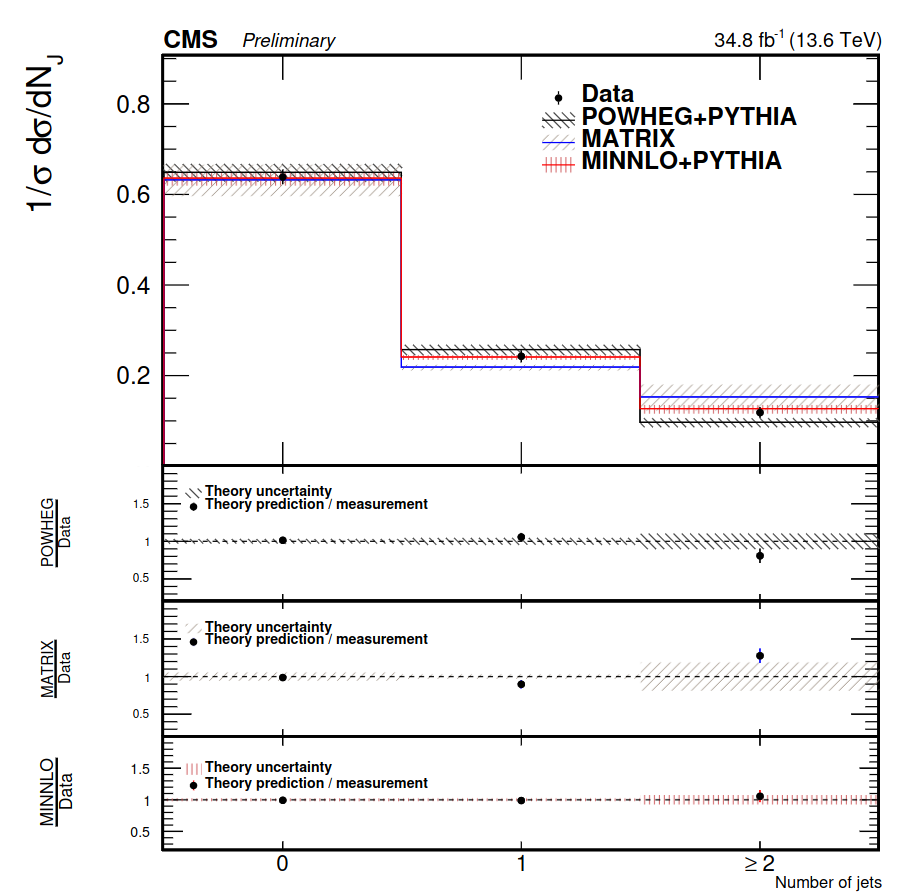
Figure 2: The upper panel shows the normalized cross section measurement as a function of the number of jets: 0, 1, and more than 1. The black circles represent the data (after background subtraction and unfolding of the detection effects). The lines represent predictions from two computations. The two lower panels show the ratio between the theoretical predictions and the measurement. In all panels, the vertical bars represent the uncertainty of the measurement and the shaded bands depict the uncertainty of the prediction.
Read more about these results:
-
CMS Paper (SMP-24-001) "Measurement of W+W− inclusive and differential cross sections in pp collisions at 13.6 TeV with the CMS detector"
-
Display of collision events: CERN CDS
-
@CMSExperiment on social media: LinkedIn - facebook - twitter - instagram
- Do you like these briefings and want to get an email notification when there is a new one? Subscribe here